en|de

OpenCV practice: OCR for the electricity meter

Martin Kompf

OpenCV (Open Computer Vision) is a powerful and comfortable environment for the realization of a variety of projects in the field of image processing. This tutorial introduces some aspects of OpenCV based on a practical application - the reading of an electricity meter.
In many homes there are still electricity meters with a mechanical counter that do not provide a direct, standardized interface for reading the consumption of electrical energy with a computer. One way to gain access to this data anyway, consists in the optical detection of the counter with a video camera and the subsequent character recognition (OCR - Optical Character Recognition). The tutorial describes the implementation of this use case with OpenCV. The resulting program even runs on a Raspberry Pi.

Content

Content
Workflow
Installing OpenCV
Image capture
cv::Mat
Image processing
Rotation
Recognition of edges and lines
Contours
Machine Learning
Persistence
Plausibility check
Data storage and analysis
Main program
Conclusion
Interesting links

Workflow

Fig. 1: Program flow

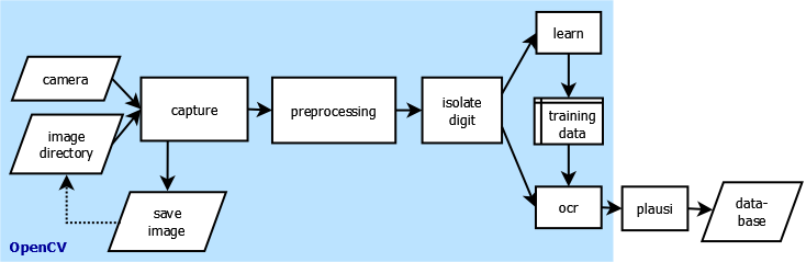
Fig. 1 shows the basic program flow. At the beginning the image of the electricity meter is recorded at specified intervals by a video camera. After imaging, the program can alternatively save the image in the file system to read it later from there. This is very useful for development and testing because you don't have always to connect the camera.

The image goes through pre-processing next. This step should change and optimize the image so that in the next step the detection and isolation of the individual digits of the counter is possible.

The extracted images of the digits then enter the character recognition (OCR). It has to, however, trained first with a set of all possible characters (the digits 0 through 9) interactively. This produces a set of training data, which is stored in a file. During normal operation, the OCR loads this training data and can thus classify an unknown character.

This classification is done with a certain error. Before further processing, it therefore makes sense to check the readings for plausibility. If it is passed, then the detected counter value together with the current time is stored in a database. With the data stored here one can make later evaluations, such as the generation of graphics with the hourly, daily and weekly power consumption. Plausibility check and database are not implemented with OpenCV, but are also mentioned in this tutorial for the sake of completeness.

Installing OpenCV

OpenCV is part of many Linux distributions, especially of Raspbian, Debian and Ubuntu. The runtime components are available as dynamic libraries and can be installed with the package manager. The developer of OpenCV programs can choose the programming language between C ++ and Python. This tutorial uses C++ and thus relies on a working C++ development environment under Linux and the corresponding basic knowledge in software development with C++.

On Debian-based distributions, the installation of the components required to develop C++ OpenCV programs takes place with

apt-get install libopencv-dev

This requires root privileges, which are to gain usually by putting sudo in front of the command. The so installed version is not the latest one, which can be downloaded at OpenCV Downloads. However, only the version 2.3.1 is required for this tutorial, therefore the version installed with the package manager on a recent Linux distribution should be quite sufficient. The software has been tested against OpenCV 2.3.1 (on Debian wheezy), 2.4.1 (Raspbian) and 2.4.8 (Ubuntu 14.04).

Although the finished program is running on a Raspberry Pi, it is recommended to use a more powerful computer for developing and testing. Otherwise the iterative compiling and testing of the source code consumes too much time in the long run. It makes sense to choose a Debian-based distribution for its operating system, since it is similar to Raspbian.

In any case, one should visit the OpenCV documentation page after the installion and download the Reference Manual for the appropriate version. The reference for the latest stable version is also available online.

The source code of the fully functional sample program developed in this tutorial is available as project emeocv (Electric meter with OpenCV) on Github. A local copy is created by

git clone https://github.com/skaringa/emeocv.git

The program requires additional components for logging (log4cpp) and data storage (RRDtool), which may be installed by

apt-get install rrdtool librrd-dev liblog4cpp5-dev

Then you can try to compile and link the program:

cd emeocv
make

If this is working without errors, then all required components are on board.

Image capture

A USB webcam captures the image of the electricity meter (Fig. 2). With OpenCV only two lines of source code are required for this. Similarly easy is the reading of an image from a file. Since the program is designed to deal with both input methods, an object oriented approach is useful here. Let us define a base class ImageInput, which keeps the image and the time stamp of image acquisition.

For the complete code look at the above-mentioned Git-Repository, the abbreviated definition is:

#include <opencv2/imgproc/imgproc.hpp>
#include <opencv2/highgui/highgui.hpp>

class ImageInput {
public:
    virtual bool nextImage() = 0;

    virtual cv::Mat & getImage();
    virtual time_t getTime();
    virtual void saveImage();

protected:
    cv::Mat _img;
    time_t _time;
};

The derived classes DirectoryInput and CameraInput each implement the method nextImage(), which is responsible for reading the image:

class DirectoryInput: public ImageInput {
public:
    virtual bool nextImage();
};

class CameraInput: public ImageInput {
public:
    CameraInput(int device);
    virtual bool nextImage();

private:
    cv::VideoCapture _capture;
};

DirectoryInput takes care of reading an image from a file, the essential OpenCV code is:

bool DirectoryInput::nextImage() {
    // read image from file at path
    _img = cv::imread(path);
    return true;
}

The capture of an image with the camera assumes the existence of a video capture object. The constructor CameraInput opens the input channel by VideoCapture.open(). Parameter is the serial number of the camera, starting with zero:

CameraInput::CameraInput(int device) {
    _capture.open(device);
}

bool CameraInput::nextImage() {
    // read image from camera
    bool success = _capture.read(_img);
    return success;
}

For testing purposes you might want to save the captured image into a file. The method saveImage of the base class handles this:

void ImageInput::saveImage() {
    //std::string path = ...
    if (cv::imwrite(path, _img)) {
        log4cpp::Category::getRoot() << log4cpp::Priority::INFO << "Image saved to " + path;
    }
}

Another frequently used function is to display an image. OpenCV also provides a one-liner for this task to disburden the developer from dealing with operation system-specific characteristics:

  cv::imshow("ImageProcessor", _img);

The first argument is the name of the window. So different calls of imshow may run into the same window. For a simple user interaction the method waitKey is available:

  int key = cv::waitKey(30);

It is waiting for 30 milliseconds for a user input and returns the pressed key.

With these methods it is already possible to write a simple program, which captures an image with the camera at defined intervals, displays and stores it in a file:

ImageInput* pImageInput = new CameraInput(0);
pImageInput->setOutputDir("images");
while (pImageInput->nextImage()) {
    pImageInput->saveImage();
    cv::imshow("Image", pImageInput->getImage());
    int key = cv::waitKey(1000);
    if (key == 'q') break;
}

As camera serves a simple USB Video Class (UVC) webcam with a resolution of 640x480 pixels. This is quite sufficient for the use case. A higher resolution should not enhance the accuracy of the character recognition, but uses a lot more memory and CPU time for image processing, which are very limited resources just on the Raspberry Pi.

Much attention must be paid to the subject of lighting. Since the electricity meter is located in a closet in the cellar, an artificial lighting is required. In this course, a low energy consumption is a top priority. In the project, a flexible LED light strip with a consumption of about 1.5 watts is used. It is powered by a wall power supply with 12 volts DC output.

The light should be in no way addressed directly to the electricity meter. This inevitably leads to reflections on the cover plate, which make subsequent image processing impossible, if they exactly are located on a digit of the counter and outshine them. The use of a diffuser between the light source and counter has proven itself. For this I use parts of a disused plastic canister. His milky white, semi-transparent material is well suited for producing a diffuse illumination.

cv::Mat

At this point, take a brief look at the way how OpenCV stores an image. Both imread() for reading an image from a file and VideoCapture.read() for capturing the image from a camera produce an object of type cv::Mat.

The namespace prefix cv encapsulates most classes and functions of OpenCV to avoid name collisions with other libraries. Mat is a n-dimensional array, or matrix, which can be used for storing different things. An important feature is the built-in memory management. You can copy and reuse it, without having to worry about the allocation or freeing of memory. In particular, copy is also a very cheap operation, because only a reference counter is incremented rather than duplicating the entire storage area. Does one need a true copy of a Mat object, then its member function clone() should be used.

In our example, the Mat object _img contains the captured image. By default, imread() and VideoCapture.read() produce images in the BGR (blue-green-red) color space. This is identical to the known RGB color model, only with an inverted arrangement of the color channels in the memory. The model describes each pixel of the image with three independent intensity values for blue, green and red.

Another often used color model is Grayscale, encoding each pixel with a single gray value. In this case, cv::Mat is a two-dimensional matrix, while it is three-dimensional in the BGR color space. The detection of the color model of an image is possible with the function channels(). It returns the value three for BGR and one for Grayscale.

A frequently used function is the transformation of a BGR image to grayscale with the method cvtColor:

cv::Mat color, gray;
color = cv::imread(filename);
cvtColor(color, gray, CV_BGR2GRAY);

Image processing

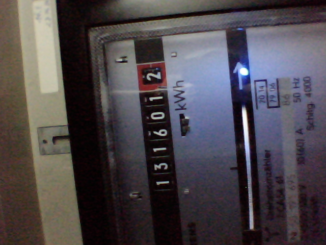
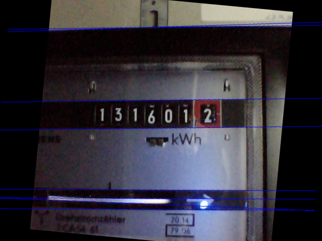
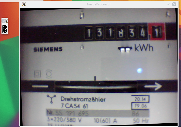
Fig. 2: The image captured by the camera is twisted and dark

A snapshot of the electricity meter is now in a cv::Mat object. Before we can venture out to the character recognition of the counter, the algorithm has to identify and extract the single digits of the counter. Let us look at an image of the electricity meter shot with the camera (Fig. 2): What our lifetime trained brain manages with ease, is a huge problem for the "unskilled" computer. What criterion distinguishes the character "0" of the mechanical counter from the "0" in the frequency specification 50 Hz? A possible algorithm for extracting the relevant information from the image we want to work out in the following.

The class ImageProcessor encapsulates all the methods required to do so. The abbreviated definition is:

class ImageProcessor {
public:
    void setInput(cv::Mat & img);
    void process();
    const std::vector<cv::Mat> & getOutput();
private:
    cv::Mat _img;
    cv::Mat _imgGray;
    std::vector<cv::Mat> _digits;
};

With setInput() you pass the image to be processed. The function process() performs the complete processing. On success getOutput() provides the result. It consists of a vector of images. Each image contains a single digit of the counter. If the algorithm was successful, then the length of the vector should be exactly seven.

The function process() delegates the individual processing steps to other private functions. The procedure is the same for each image:

Conversion into a grayscale image
Rotation, so that the digits of the counter are on a horizontal line
Locate and cut out each digit

void ImageProcessor::process() {
    _digits.clear();

    // convert to gray
    cvtColor(_img, _imgGray, CV_BGR2GRAY);

    // initial rotation to get the digits up
    rotate(_config.getRotationDegrees());

    // detect and correct remaining skew (+- 30 deg)
    float skew_deg = detectSkew();
    rotate(skew_deg);

    // find and isolate counter digits
    findCounterDigits();
}

Rotation

After converting the image to grayscale, the algorithm should rotate the image to such an extent that the seven digits of the counter are on a horizontal line. So their identification is much easier: Seven horizontally arranged, bright contours.

The rotation of an image does the cv::warpAffine() function by means of an affine transformation. These are - to put it simply - such changes of the image, in which all parallel lines even after the transformation are still parallel. These include translation, rotation and scaling. All of these transformations can be described using a transformation matrix. When multiple affine transformations are to applied to the same image, then it often makes sense for performance reasons to first multiply each transformation matrix step by step and make the actual transformation of the image at the very end.

The rotation of the image by a predetermined angle is outsourced into the function rotate():

void ImageProcessor::rotate(double rotationDegrees) {
    cv::Mat M = cv::getRotationMatrix2D(
      cv::Point(_imgGray.cols / 2, _imgGray.rows / 2),
      rotationDegrees, 1);

    cv::Mat img_rotated;
    cv::warpAffine(_imgGray, img_rotated, M, _imgGray.size());
    _imgGray = img_rotated;
}

For the construction of the rotation matrix - in addition to the angle - the point of rotation is required. For this we calculate the center of the image from the number of its columns (cols) and rows (rows).

Now we have the tools at hand to straighten the image. What's missing is the determination of the rotation angle. That is taken place in two steps. The reason for this lies in the mechanical construction of mounting suspension of the camera:

The USB webcam has a clip for attaching it to a tripod and a ball joint which allows pivoting about all three spatial axes within certain limits. By means of the clip the camera is attached to a vertical bar. This means that all the images are rotated in principle by 90 degrees counterclockwise. These design-related rotation can first be undone by specifying a fixed angle:

    // initial rotation to get the digits up
    rotate(_config.getRotationDegrees());

The required angle is configurable. The configuration is encapsulated by the _config object - to that later more. In the example, the angle has a value of 270° (corresponds to -90°) to compensate the construction-dependent rotation.

After that, the counter positions are still not aligned exactly horizontally. This is due to the adjustment of the ball joint. Although you could try to align the camera precisely by rotating the joint under constant visual control of the captured image. But this is likely to be a time-consuming and annoying business. It would be better if we could detect and compensate the remaining alignment errors by software!

Recognition of edges and lines

Our eye is not based on reading of the count (for example, Fig. 2) by absolute brightness or color values. The ganglion cells in the retina are rather wired so that they respond to a high contrast. Thus, the brain is able to identify edges and lines very quickly and finally to determine the external shape of the meter and and the individual numbers in a wide range of brightness.

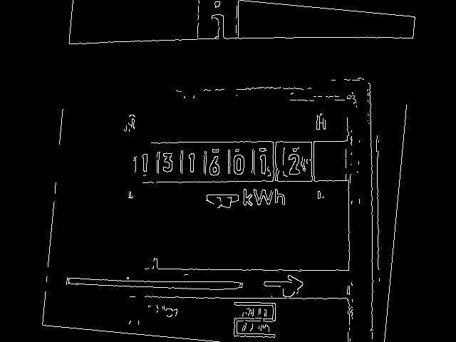
Consequently. a large part of OpenCV is dedicated to the identification of edges and lines. A useful routine for many situations is the Canny algorithm. Canny() receives the grayscale image as input and provides an image with the detected edges as output similar to Fig. 3:

/**
 * Detect edges using Canny algorithm.
 */
cv::Mat ImageProcessor::cannyEdges() {
    cv::Mat edges;
    // detect edges
    cv::Canny(_imgGray, edges, _config.getCannyThreshold1(), _config.getCannyThreshold2());
    return edges;
}

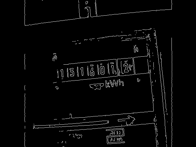
Fig. 3: The Canny algorithm detects edges

The two threshold parameters of Canny depend on the lighting and the contrast of the image and therefore are outsourced to a configuration file. High contrast images require high threshold values. For Fig. 2, the values 200 and 250 were used. An alternative tested lighting situation generated images with lower contrast (Fig. 4), this results in the values 100 and 200 for the thresholds. One has to try something around to find the optimal parameters.

Fig. 4: Recording with brighter lighting, but lower contrast requires the adaptation of Canny thresholds

Unimportant details have now largely disappeared from the edge image . However, all relevant information for the process are still in place: Firstly, the seven counter digits (we will care about them later). On the other hand several parallel lines are seen, for example, the limitations of the meter housing, counter and counting ring. The deviation of the horizontal lines is exactly the angle that you need to align the image.

That which recognizes our eye immediately as a line, is for OpenCV only an array of bright pixels on a black background at this time. To identify lines, we performs a Hough transform next by means of cv::HoughLines():

/**
 * Detect the skew of the image by finding almost (+- 30 deg) horizontal lines.
 */
float ImageProcessor::detectSkew() {
    cv::Mat edges = cannyEdges();

    // find lines
    std::vector<cv::Vec2f> lines;
    cv::HoughLines(edges, lines, 1, CV_PI / 180.f, 140);

The here hardcoded threshold of 140 is the number of votes that an edge needs to be identified as a line. The larger the value, the longer must be the continuous line. If you observe inaccuracies in the determination of the angle in detectSkew(), then it makes sense to experiment with this value first.

HoughLines() returns the vector lines containing all detected lines. Each element of lines in turn is a vector with two elements. The first element is the distance of the line from the upper left corner of the image, the second is the angle relative to the vertical.

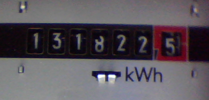
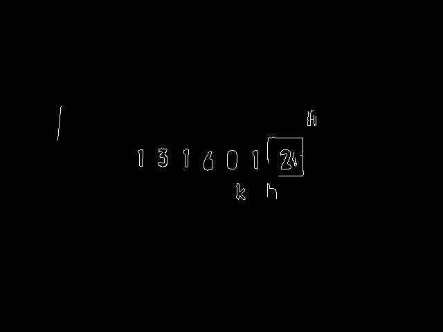
This angle is exactly what we need. But from what line? There are probably the vertical lines included in the result too. If the maximum compensable rotation error is limited to 30°, then you can now filter out all interesting lines with this criterion and compute the average over the angle. It should also be noted that HoughLines() returns the angle in radians, while rotate() requires the rotation angle in degrees. Fig. 5 shows the finally aligned camera image with the lines used for angle determination.

    // filter lines by theta and compute average
    std::vector<cv::Vec2f> filteredLines;
    float theta_min = 60.f * CV_PI / 180.f;
    float theta_max = 120.f * CV_PI / 180.0f;
    float theta_avr = 0.f;
    float theta_deg = 0.f;
    for (size_t i = 0; i < lines.size(); i++) {
        float theta = lines[i][1];
        if (theta > theta_min && theta < theta_max) {
            filteredLines.push_back(lines[i]);
            theta_avr += theta;
        }
    }
    if (filteredLines.size() > 0) {
        theta_avr /= filteredLines.size();
        theta_deg = (theta_avr / CV_PI * 180.f) - 90;
    }
    return theta_deg;
}

Fig. 5: The correctly oriented image with guides

Contours

Now it can go on to the identification and extraction of each digit of the counter. The starting point are the edges obtained with Canny() from the straightened image (Fig. 6).

Fig. 6: Edge image with the correct orientation

To recognize the digits we use the contour detection of OpenCV, which is implemented in the function findContours(). Since this function changes the image matrix, we create a copy of the edge image with clone() beforehand:

/**
 * Find and isolate the digits of the counter,
 */
void ImageProcessor::findCounterDigits() {
    // edge image
    cv::Mat edges = cannyEdges();
    cv::Mat img_ret = edges.clone();

    // find contours in whole image
    std::vector<std::vector<cv::Point> > contours, filteredContours;
    std::vector<cv::Rect> boundingBoxes;
    cv::findContours(edges, contours, CV_RETR_EXTERNAL, CV_CHAIN_APPROX_NONE);

The found contours are returned in the vector contours. Each element represents a single contour, which is defined as a vector of points. The CV_RETR_EXTERNAL parameter instructs findContours() to deliver only the outer boundaries.

From the result, which even now contains all possible contours, we have to filter out the interesting digits. This is done in two steps: first, we filter out the contours depending on the size of their bounding boxes:

    // filter contours by bounding rect size
    filterContours(contours, boundingBoxes, filteredContours);

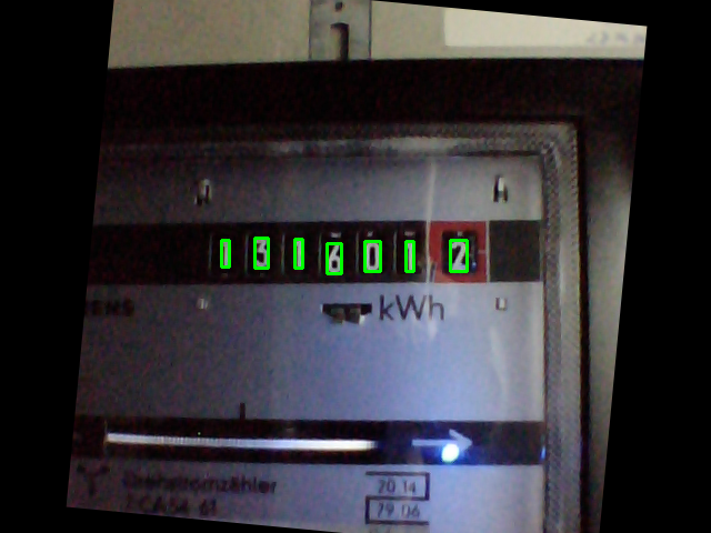
The function filterContours() (complete source code in GitRepo) iterates over the contours vector and calls cv::boundingRect() for each element. It returns an object of type cv::Rect, describing the rectangle of the outer enclosure of the contour. The algorithm then inspects the height and width of the bounding box. The height must lie within predetermined, configurable limits and always be greater than its width. Fig. 7 shows the result of the filtering.

Fig. 7: The filtered contours contain all digits of the counter and still some disturbances

The image now contains still some disturbances in addition to the usable digits. To identify the latter, we evaluate in the second step the y-positions and heights of the calculated bounding boxes. The algorithm attempts to find the largest number of equal sized contours on a horizontal line from all possible combinations of bounding boxes. The resulting vector alignedBoxes contains then most likely the bounding boxes of the digits, because no other group of contours is so significantly aligned.

    // find bounding boxes that are aligned at y position
    std::vector<cv::Rect> alignedBoundingBoxes, tmpRes;
    for (std::vector<cv::Rect>const_iterator ib = boundingBoxes.begin();
      ib != boundingBoxes.end(); ++ib) {
        tmpRes.clear();
        findAlignedBoxes(ib, boundingBoxes.end(), tmpRes);
        if (tmpRes.size() > alignedBoundingBoxes.size()) {
            alignedBoundingBoxes = tmpRes;
        }
    }

The result should contain the digits in their arrangement from left to right, therefore the bounding boxes are sorted according to their x-position:

    // sort bounding boxes from left to right
    std::sort(alignedBoundingBoxes.begin(), alignedBoundingBoxes.end(), sortRectByX());

With this information you can now cut out the individual digits from the image. The operator () of cv::Mat is responsible for this, it gets the "region of interest" (ROI) as parameter. Optionally cv::rectangle() draws the ROIs as green boxes into the original image (Fig. 7). This is very helpful when adjusting the camera and light source.

    // cut out found rectangles from edged image
    for (int i = 0; i < alignedBoundingBoxes.size(); ++i) {
        cv::Rect roi = alignedBoundingBoxes[i];
        _digits.push_back(img_ret(roi));
        if (_debugDigits) {
            cv::rectangle(_img, roi, cv::Scalar(0, 255, 0), 2);
        }
    }
}

The detected bounding boxes of the digits plotted are into the original image

Fig. 7: The detected bounding boxes of the digits are plotted into the original image

Machine Learning

Each component of the vector _digits contains the edge image of a single digit (Fig. 8).

Fig. 8: A gallery of exemplary images of digits

The computer derives the information which character is represented by an image by means of optical character recognition (OCR). One technique often used for this is machine learning. In a first step, the systems is trained with various test data. This results in a model which describes a mapping from data (images) into information (character encoding). Using this model, the trained system then can transform unknown data into the desired information during the second step.

There are a variety of algorithms for machine learning, of which OpenCV implements a great extent. Choosing the right algorithm for a specific problem requires a lot of experience and knowledge. In the following one of the simplest algorithms is used: K-nearest neighbors. It is known to be very accurate but on the other hand it consumes a lot of CPU time and memory. These drawbacks are not so critical to our application - there is sufficient time, because the counter is not rotating very fast. Memory is limited to the Raspberry Pi though, but it should be sufficient for the small size of the model that has to detect only ten digits.

For the implementation of training and character recognition, the class KNearestOcr is responsible:

class KNearestOcr {
public:
    int learn(const cv::Mat & img);
    char recognize(const cv::Mat & img);

    void saveTrainingData();
    bool loadTrainingData();
private:
    cv::Mat prepareSample(const cv::Mat & img);
    void initModel();

    cv::Mat _samples;
    cv::Mat _responses;
    CvKNearest* _pModel;
};

The routines for machine learning may work with various input data - not just with pictures. The preparation of the input data is also called "Feature Extraction". It should only produce such data that is relevant for the learning process. This has been done in our image pre-processing very well: It produced only the contours of the digits without any background and color information. The feature extraction can therefore be very easy at this point: First, it brings all the digits on the uniform size of 10x10 pixels with cv::resize(). Since K-nearest neighbors works with one-dimensional vectors of floating point numbers, the functions reshape() and convertTo() are used to convert the image matrix into this format:

/**
 * Prepare an image of a digit to work as a sample for the model.
 */
cv::Mat KNearestOcr::prepareSample(const cv::Mat& img) {
    cv::Mat roi, sample;
    cv::resize(img, roi, cv::Size(10, 10));
    roi.reshape(1, 1).convertTo(sample, CV_32F);
    return sample;
}

The learning routine then builds the two fields _samples and _responses. _samples contains all features (the result of prepareSample), which have passed the training process successfully. The field _responses contains the associated "Reply" of the coach for each feature - that is the corresponding number. Implementing the interactive training routine is amazingly simple:

/**
 * Learn a single digit.
 */
int KNearestOcr::learn(const cv::Mat & img) {
    cv::imshow("Learn", img);
    int key = cv::waitKey(0);
    if (key > '0' && key < '9') {
        _responses.push_back(cv::Mat(1, 1, CV_32F, (float) key - '0'));
        _samples.push_back(prepareSample(img));
    }

    return key;
}

First cv::imshow() shows the image of the digit. Then cv::waitKey() waits for the input of the coach. If this is a valid digit, then it is written together with the associated feature to _responses and _samples.

The user can terminate the training process at any time with the key 'q' or 's' (see also learnOcr() in main.cpp). In the case of 's' the method saveTrainingData() writes the fields _samples and _responses into a file. We will discuss this in the section persistence below in more detail.

During regular operation KNearestOcr::loadTrainingData() first loads this file and initializes the model:

/**
 * Initialize the model.
 */
void KNearestOcr::initModel() {
    _pModel = new CvKNearest(_samples, _responses);
}

The model is now able to classify any image that was prepared with prepareSample() by determining the closest neighbor feature and returning the associated, learned response.

Our recognize() routine even goes a little further: It uses find_nearest() to determined the two nearest neighbors and their distance to the original. Only when both values match, and the distance is below a threshold, the function returns a valid character. You should definitely dedicate some time to determine the configurable threshold ocrMaxDist. Small values lead to the rejection of actually correctly identified values and cause longer gaps in the captured data. In contrast, a too high value produces too many errors in the results. For my specific environment I've been found an optimum using the value 600000.

/**
 * Recognize a single digit.
 */
char KNearestOcr::recognize(const cv::Mat& img) {
    char cres = '?';
    cv::Mat results, neighborResponses, dists;
    float result = _pModel->find_nearest(
      prepareSample(img), 2, results, neighborResponses, dists);

    if (0 == int(neighborResponses.at<float>0, 0) - neighborResponses.at<float>0, 1))
          && dists.at<float>0, 0) < _config.getOcrMaxDist()) {

        cres = '0' + (int) result;
    }
    return cres;
}

Persistence

The program requires the ability to store data persistently in the file system and to load them again from there at various points. These are the trained model for the character recognition and a configuration file with different parameters. The first requirement on the persistence layer is therefore the ability to deal with structured data such as cv::Mat. Second, the configuration file should be simple and intuitive to edit by the user in a text editor.

OpenCV provides with cv::FileStorage an interface that meets both requirements. It allows saving and loading the most built-in OpenCV simple and complex data types as well as numerical and textual standard C data types. The file format can be chosen from XML or YAML, this is controlled via the file extension. For emeocv I chose YAML because it is more compact and easier to read.

The reading and writing of data can be performed with C++ streams. At first a textual key is written and then the data. The key is required to assign the data correctly during reading. So the storing and reading of the trained data model in KNearestOcr only needs a minimal number of lines of code:

/**
 * Save training data to file.
 */
void KNearestOcr::saveTrainingData() {
    cv::FileStorage fs(_config.getTrainingDataFilename(), cv::FileStorage::WRITE);
    fs << "samples" << _samples;
    fs << "responses" << _responses;
    fs.release();
}

/**
 * Load training data from file and init model.
 */
bool KNearestOcr::loadTrainingData() {
    cv::FileStorage fs(_config.getTrainingDataFilename(), cv::FileStorage::READ);
    if (fs.isOpened()) {
        fs["samples"] >> _samples;
        fs["responses"] >> _responses;
        fs.release();

        initModel();
    } else {
        return false;
    }
    return true;
}

Similarly works the reading of the configuration file config.yml in class Config:

void Config::loadConfig() {
    cv::FileStorage fs("config.yml", cv::FileStorage::READ);
    if (fs.isOpened()) {
        fs["rotationDegrees"] >> _rotationDegrees;
        fs["digitMinHeight"] >> _digitMinHeight;
        // and so on

    } else {
        // no config file - create an initial one with default values
        saveConfig();
    }
}

Plausibility check

As seen in the recognize() method of the OCR, the character recognition already makes a decision whether the recognition error falls below a certain threshold. If it is too high, then recognize returns the character '?'. However, this test is sometimes insufficient. It does happen that the OCR confuses the characters 0 and 8. Another critical point is the fact that the digits of the counter don't switch in a defined way, but rotate slowly into the field of view from bottom to top. If then, for example, only the upper part of digit 2 is visible, then it resembles the digit 7 and leads to false positives.

OCR programs for text recognition use a dictionary for this reason. This not only allows the exclusion of obviously nonsensical letter combinations, but in many cases an automatic correction. Unfortunately, this approach fails to detect a numerical count - there is no such dictionary.

However, one can define a set of rules to check the plausibility of the counter value provided by the OCR before further processing. The implementation is in the class Plausi. It no longer uses OpenCV, but should be mentioned here for the record. The implemented rules are:

A count is made of exactly seven significant digits.
Since the counter never turns backwards, the current value must not be smaller than the previous.
By forming the difference between two meter readings and dividing by the elapsed time we obtain the average power rating $P = \frac{W}{t} = U I$ . This power can not be greater than the maximum value predetermined by the fuse of the circuit. For example, if a household powered with 220 volt is protected by a 50 amp fuse, then P can't be larger than 11 kilowatts.

The 2nd and 3rd check rules that the Plausi class has to buffer the last meter reading and its time stamp. In practice, it has then shown that the consideration of only two values is sometimes not enough and in particular produces upward spikes. Therefore Plausi stores the last eleven values in a queue. Only if all these values satisfy the validity checks, the central value of the queue is forwarded.

Data storage and analysis

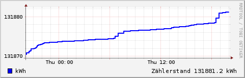
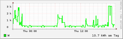
The further processing of valid meter readings is also no longer an issue of OpenCV. In my application I have decided to store count and power consumption in a Round Robin Database.

A meaningful temporal resolution of the consumption values vary with their age: The latest measurements should be dissolved as precisely as possible - about a minute. If looking back one week however I'm only interested in the cumulative daily values and for the whole year weekly averages are quite sufficient. For this reason a round-robin database with automatic data consolidation in the form of rrdtool has been chosen.

The creation of the database is done with the script create_rrd.sh:

rrdtool create emeter.rrd \
--no-overwrite \
--step 60 \
DS:counter:GAUGE:86400:0:1000000 \
DS:consum:DERIVE:86400:0:1000000 \
RRA:LAST:0.5:1:4320 \
RRA:AVERAGE:0.5:1:4320 \
RRA:LAST:0.5:1440:30 \
RRA:AVERAGE:0.5:1440:30 \
RRA:LAST:0.5:10080:520 \
RRA:AVERAGE:0.5:10080:520

The parameter --step 60 sets the basic time interval to 60 seconds = 1 minute. Then you define two data sources DS: counter is used to record the meter reading (which is the work done W) and consum stores the electric power P. Since it is of type DERIVE, it automatically makes a differentiation of values to be stored for the period.

$P = \frac{W}{t}$

The definitions of the Round Robin Archives (RRA) determine the number and retention of data: The minute values are kept three days (according to 4320 values), the consolidated daily values are kept for 30 days and the week values 520 weeks (or about 10 years).

Two RRAs are defined for each period. They differ in their consolidation function: The consolidation LAST is in charge of the counter, because here interested indeed the last measured value. In contrast, for consumption you don't want the last value, but the average - this is why the AVERAGE function comes into play.

The command creates the file emeter.rrd with a size of about 150 kilobytes. No matter how much data you put into - since it is a round-robin database, the size does not change!

The function update() of the class RRDatabase is responsible for writing the values into the database:

int RRDatabase::update(time_t time, double counter) {
    char values[256];
    snprintf(values, 255, "%ld:%.1f:%.0f",
      (long)time, counter/* kWh */, counter * 3600000. /* Ws */);

    char *updateparams[] = { "rrdupdate", _filename, values, NULL };

    rrd_clear_error();
    int res = rrd_update(3, updateparams);
    return res;
}

The function receives a time stamp and a meter reading. The snprintf() statement builds an update string for rrdtool. The first two parameters are time stamp and meter reading. The third parameter is also the meter reading. It goes into the data source consum that we have declared as type DERIVE during creation of the database. Therefore it is differentiated automatically, one second is used as a time unit. Because the count has the unit kilowatt hours (kWh), it is recommended to convert it into watt seconds (Ws). This causes that the data source consum contains the average power in the unit watt (W).

An outstanding feature of RRDtool is the possibility of direct generation of graphics. For this, the data collection should run for a few hours. Then a graphic with the consumption during the last 24 hours may be produced like this:

rrdtool graph consum.gif \
  -s 'now -1 day' -e 'now' \
  -Y -A \
  DEF:consum=emeter.rrd:consum:AVERAGE \
  LINE2:consum#00FF00:W \
  CDEF:conskwh=consum,24,*,1000,/ \
  VDEF:conspd=conskwh,AVERAGE \
  'GPRINT:conspd:%.1lf kWh per day'

Fig. 9: History of meter reading and consumption over one day

Other examples can be found in the subdirectory www of the Git repository. This directory contains some HTML pages and Perl scripts to build a minimal web application that presents counter and consumption figures for various periods on the intranet.

Main program

The main program in the file main.cpp takes over the coordination of the components described. It is controlled via command line parameters, a short explanation provides the option -h:

Usage: emeocv [-i <dir>|-c <cam>] [-l|-t|-a|-w|-o <dir>] [-s <delay>] [-v <level>]

Image input:
  -i <image directory> : read image files (png) from directory.
  -c <camera number> : read images from camera.

Operation:
  -a : adjust camera.
  -o <directory> : capture images into directory.
  -l : learn OCR.
  -t : test OCR.
  -w : write OCR data to RR database. This is the normal working mode.

Options:
  -s <n> : Sleep n milliseconds after processing of each image (default=1000).
  -v <l> : Log level. One of DEBUG, INFO, ERROR (default).

The input is selected by -i (Image directory) or -c (camera). In addition, the specification of the desired operation is required. One starts usually when the camera is connected with:

emeocv -c0 -a -s10 -vINFO

This is used to adjust the camera and light. The program opens a window to display the image recorded by the camera. The user can switch with the keys r and p between the original and the pre-processed image. By means of

emeocv -c0 -o images -s10000

a directory can be filled with images taken by the camera every 10 seconds. These images can be inspected offline:

emeocv -i images -a -s0 -vINFO

The aim is to achieve a correct segmentation of each digit of the counter, as it can be seen in Fig. 7. This is achieved primarily by modifying the configuration parameters in config.yml. The parameters are not documented, a basic understanding of the operation and the source code are therefore an essential prerequisite for this step!

If successful, it is time to train the OCR:

emeocv -i images -l

It opens two windows. In the big one you can see the original image, in the smaller - easily overlooked - the figure to be trained appears (Fig. 10).

Abb. 10: In training mode two windows open, in the smaller one is the number to be trained.

The training result is checked with:

emeocv -i images -t -s0

For normal operation, the database should be created first as described above. The acquisition program ideally runs in the background:

nohup emeocv -c0 -w -s10000 -vINFO &

With -s10000 the data acquisition takes place every 10 seconds. This leaves enough time for other tasks to the CPU of the Raspberry Pi. But the intervals should be not to large, because this increases the likelihood that an incomplete number is at the last counter digit and a correct detection isn't possible.

The -v option controls the output of messages to the log file emeocv.log. The logging isn't described in the present paper, the underlying techniques and frameworks (here: log4cpp) should be known.

Conclusion

A prototype is working on a Raspberry Pi Model B for several weeks and meets the intended use case "Monitoring of power consumption in a private household" satisfactory. Impressive is the low effort for hardware. In addition to the Raspberry Pi only a simple USB webcam is required. The exciting part of the processing is implemented entirely in software. The main work - image capture, processing and character recognition - is done by OpenCV.

This publication is intended to stimulate further trials - any feedback is welcome! In no case is this a step-by-step instruction or even a finished program for the end user. This would require to implement more algorithms, such as tolerance to changing light conditions, automatic determination and adjustment of configuration parameters and a better character recognition for different types of digits.

Interesting links

emeocv - Repository on Github
OpenCV
Raspberry Pi Wiki at eLinux.org
Raspberry Pi Foundation
RRDtool - OpenSource Data Acquisition and Visualization tool